


When working with a large amount of data in a spreadsheet in Microsoft Excel, it can become difficult to figure out which category or heading the data in a cell corresponds to, especially when the rows or columns you want to compare are far away from each other. Oftentimes you may find yourself scrolling up and down a sheet just to see the column headers for the cells you’re examining.
An easy solution to this problem is to freeze header rows or columns on your sheet in Excel. A frozen row or column stays visible as you scroll through the rest of the document, letting you easily keep in view the headings for the data you’re working with.
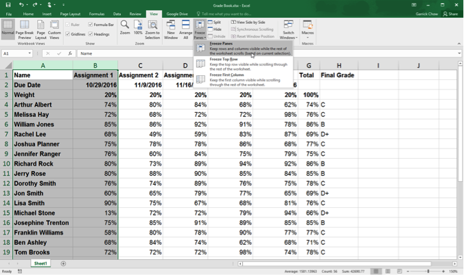
To do this, go to the View tab and click the Freeze Panes button. That gives you the choices of Freeze Panes, Freeze Top Row, and Freeze First Column.
So if, for example, you want to keep the top row of your sheet stationary, choose Freeze Top Row. After that it will remain onscreen and in place as you scroll vertically through the rest of the document.
Or, if you want to freeze more than first row or column, first select the rows or columns you want to freeze. Then click the Freeze Panes button and choose Freeze Panes. That locks all the selected rows or columns in place.
Note that you can’t freeze the top row and top column simultaneously. Picking one automatically unfreezes the other. To allow the entire sheet scroll normally again, click the Freeze Panes button and choose Unfreeze Panes.
Again, the ability to freeze rows and columns can really come in handy when working with long and dense spreadsheets.
Want to fully unlock the power of Microsoft Excel? Check out all of our LinkedIn Learning courses on the topic.

Topics: Productivity tips
Related articles